First Mesh Walkthrough

In this walkthrough, we will go through the process of creating your first dripline mesh. A “mesh” refers to an AMQP message broker and all of the services which are connected to it. In most cases, this is the same as the controls for a particular system.

Here we will create a very simple mesh, which includes:

1. a rabbitmq broker for communication (this is a 3rd party application)

2. a trivial service, which can be thought of as representing a simple instrument

3. a very simple PostgreSQL database for storing values (this is a 3rd party application)

4. a logging service, to store our fake sensor data in the database

5. a grafana instance, a database dashboarding tool (this is a 3rd party application)

We will try to call attention to places where decisions made here are for convenience of example, vs decisions recommended practice.

Note

If you are working through this walkthrough, you’re strongly encouraged to create a directory and write all of the files yourself, exploring the options or configurable parameters, etc. For reference, you can find a completed set of files for this example in the github repo for this documentation.

Our first big decision comes before we get started and is a question of how we will deploy and manage our software. There is more discussion in the section on process management. In this example, we will use docker-compose to define and deploy our collection of applications. If you’re not familiar with compose, please review the official documentation and work through the examples there. You should also be familiar with exec and logs subcommands, all of these will be useful throughout this guide.

Finally, before we dig in, a request:

• If something looks wrong or isn’t working, please let us know by posting an issue (or even better, for the repo and send us a PR with the correction; documentation is a group effort).

• Throughout this and all examples, we have tried to pin versions (specifically container image versions) so that the examples are reproducible over time. An excellent exercise would be to explore cases where there are newer versions and the capabilities those may enable (and again, send us a PR if you find something helpful).

Configure the message broker

The core to any dripline mesh is the AMQP message broker. In principle, dripline-compliant messages could be sent over any transport protocol you want, but in practice all available libraries are written for, and tested with AMQP (specifically RabbitMQ), so you should probably just use that. We’ll set the username and password for the default role in RabbitMQ, to be used by all of our services. In principle, RabbitMQ provides interesting and sophisticated role-based access controls features which could be leveraged, but this is not currently done. This is done with the following service block in the docker-compose file:

docker-compose.yaml

services:

  rabbit-broker:
    image: rabbitmq:3-management
    environment:
      - RABBITMQ_DEFAULT_USER=dripline
      - RABBITMQ_DEFAULT_PASS=dripline

In order for services to connect to the broker, they will need to authenticate using the username and password indicated above. The dripline libraries typically retrieve this information from an authentications file, we’ll go ahead and create that now:

authentications.json

{
    "amqp": {
        "broker": "rabbit-broker",
        "username": "dripline",
        "password": "dripline"
    },
    "postgresql": {
        "username": "postgres",
        "password": ""
    }
}

Add a dripline service

Now that we have a broker running, we will go ahead and create our first dripline service. We won’t do anythng fancy, we’ll use the built-in KeyValueStore class to create some endpoints which simply remember a value and report it back. In a more realistic use-case, the remembered value may be replaced by an interaction with some hardware, but this is nice because it runs without requiring equipment, and still demonstrates the interactions between the software components.

The compose entry

To create our dripline service, we add another object to the docker-compose definition file (under the services: block) that looks like the following:

docker-compose.yaml

  key-value-store:
    image: ghcr.io/driplineorg/dripline-python:v4.7.1
    depends_on:
      - rabbit-broker
    volumes:
      - ./authentications.json:/root/authentications.json
      - ./key-value-store.yaml:/root/key-value-store.yaml
    command:
      - dl-serve
      - -c
      - /root/key-value-store.yaml

Here we’re running a container with two files mounted in, the authentications file from the previous section, and a runtime configuration file to be discussed next. We also specify the command to run in the container (review the docker compose documentation linked above if you need help understanding the syntax).

The runtime configuration file

The configuration file is used to define the classes which need to be created to do the work of the service. The file lists those, including the configurable parameters that are passed to the __init__ functions for those classes. If you’re ever not sure what configurable parameters a class takes, you can check that function definition in the class and its base classes.

There are several important patterns for a runtime configuration file:

1. The description of classes goes in a section of the yaml file named runtime-config

2. Every class is a dictionary block, with the required keys name (uniquely naming the instance) and module (naming the class)

3. A class may include a module_path key, which indicates the path to a python source file implementing that class

4. The top-level of the runtime-config should have a class which is either a Service or a class derived from it, this class is responsible for connecting to AMQP and sending and receiving dripline messsages.

5. The Service may have an endpoints key which contains a list of dictionary blocks defining other class instances

In this case, our key-value storage service has a vanilla Service for consuming messages, and three endpoints for storing values. Taking the “peaches” endpoint as an example, we see that we’re creating an instance of the KeyValueStore class and “peaches” is its name. We’re passing in an initial_value (defined in the KeyValueStore class itself), get_on_set, log_on_set, and log_interval (from the Entity base class), and calibration (from the Endpoint base class inherited through Entity). Any other arguments those classes take in their __init__ are being left at the default values. The full configuration looks like:

key-value-store.yaml

runtime-config:
  name: my_store
  module: Service
  auth_file: /root/authentications.json
  endpoints:
        - name: peaches
          module: KeyValueStore
          calibration: '2*{}'
          initial_value: 0.75
          log_interval: 10
          get_on_set: True
          log_on_set: True
        - name: chips
          module: KeyValueStore
          calibration: 'times3({})'
          initial_value: 1.75
        - name: waffles
          module: KeyValueStore
          #log_interval: 30
          #log_on_set: True
          calibration: '1.*{}'
          initial_value: 4.00

Running and interacting

Having create the runtime configuration and added it to the compose environment, bring the the compose environment up to launch your containers. Probably the best option is to bring it up in daemon mode (with -d), but that’s up to you; I typically launch as a daemon, then use the logs subcommand with -f to follow the activity of any service I’m actively trying to debug. If you do this, you should see new output every 10 seconds when the peaches endpoints logs a new value (per the configured log_interval value).

Note

The docker-compose utility does not do sophisticated lifecycle management. Of particular relevance here, the depends_on label only indicates the order that containers should be started, it does not wait for anythign to be “ready” before moving on. It is very common that, when starting from a new or fully stopped system, RabbitMQ takes some time to start and other services fail to connect to it. The simplest solution is to simply bring everything up again, you could instead try to add sleep or automatic restart statements to deal with this automatically, but that comes with its own subtleties and is probably an indication that you should consider more sophisticated orchestration (such as k8s).

With that working, use the exec subcommand to run a second bash shell in the key-value-store container. From here, we’ll use the command line interface to interact with our new service (note that you can use the --help flag with any of these tools to find out about the full set of available options).

Use the dl-mon command (from dripline-cpp to watch the logs). The full command could be dl-mon --auth-file /root/authentications.json -b rabbit-broker -a sensor_value.#. You could similarly bind to heartbeat.# to see the regular heartbeat messages from all running services (for now we just have the one).

Use the dl-agent command to interact with an endpoint. First, we’ll check the current value of the peaches endpoing, with dl-agent --auth-file /root/authentications.json -b rabbit-broker get peaches. You should see a verbose output that includes a payload section with the current value. Now try to use the set subcommand to change the value and get it again, you should see your new value. You should also see that a new value gets logged whenever you use set, and that time-based logs have your newly assinged value.

Add historical data storage

This has all been nice for allowing us to interact with the key-value-store service. Hopefully you can see that instead of the trivial implementations of the on_get and on_set methods in the KeyValueStore class, we could implement those methods with arbitrarily complex logic and still interact with them in the same way. For this tutorial however, we set aside the question of implementing more complex interactions with hardware and focus back on software issues. In particular, as built we have a way to find out what the current value of peaches is, but not what it has been. Normally we want to catch the value logs produced and record them in a database or other long-term storage system so that they can be referenced or processed later.

The conceptual details of the logging system are discussed in the logging system section so here we jump ahead with spinning it up. Currently dripline includes an implementation for logging data into a single table (or view) in a postgreSQL database. In the rest of this section we will provision a database and a dripline service to record data into it.

Note

The database structure here is intended to serve as a minimal example and is not considered suitable for “production” or even “research and development” usage. It maximizes simplicity at the expense of all else.

Create the database

For our database, we will use the community supported postgres database container; you can find a description of the use of this container in the official documentation, hosted with the container. We create a single database with a single table for storing our endpoint values in a subdirectory next to our docker-compose.yaml file (and shortly will be mounting that directory into the container). You will need to add a database-setup file in a subdirectory called postgres_init.d. The database setup file looks like:

postgres_init.d/10_setup.sql

---
--- Create a database for our values
---

CREATE DATABASE sensor_data WITH TEMPLATE = template0;

\connect sensor_data

-- table for storing doubles
-- NOTE: this design is very bad and only used as an example for easy
--       demonstration a production system probably wants to map sensor names
--       onto IDs may want to allow annotations of entries, may want annotation
--       of sensors, etc.

DROP TABLE IF EXISTS numeric_data;
CREATE TABLE numeric_data (
  sensor_name text NOT NULL,
  "timestamp" timestamp with time zone NOT NULL default now(),
  value_raw double precision NOT NULL,
  value_cal double precision
);

We then add the postgres container to our compose file as another service. In the minimal case that looks like the following block, in a more production-like environment, the database’s storage location would need to be persistanat so that data are not lost when the container stops.

docker-compose.yaml

  postgres:
    image: postgres:16.0
    volumes:
      - ./postgres_init.d:/docker-entrypoint-initdb.d
    environment:
      # per the docs, you do *not* want to run with this configuration in production
      - POSTGRES_HOST_AUTH_METHOD=trust

Create the data logging service

Now that we have a database, we will create the data logging service to bind to alert messages with sensor data and insert that into the database. The structure is similar to other services described above, we define the dripline objects required and set the configurable parameters in a single yaml file below. Per usual, the description of these parameters are included with the classes themselves.

sensor-logger.yaml

runtime-config:
  name: sensor_data_logger
  module: PostgresSensorLogger
  auth_file: /root/authentications.json
  # SensorLogger Inits
  insertion_table_endpoint_name: values_table
  # AlertConsumer Inits
  alert_keys:
    - "sensor_value.#"
  alert_key_parser_re: 'sensor_value\.(?P<sensor_name>\w+)'
  # PostgreSQLInterface Inits
  database_name: sensor_data
  database_server: postgres
  #this is bad... waiting on a scarab update to let us pass
  #               actual details via env vars
  auths_file: "~/authentications.json"
  endpoints:
    - name: values_table
      module: SQLTable
      table_name: numeric_data
      required_insert_names:
        - sensor_name
        - timestamp
        - value_raw
      optional_insert_names:
        - value_cal

Again, following the same pattern as before, we add the dripline service to execute this configuration file to the compose configuration:

docker-compose.yaml

  sensor-logger:
    image: ghcr.io/driplineorg/dripline-python:v4.7.1
    depends_on:
      - rabbit-broker
      - postgres
    volumes:
      - ./authentications.json:/root/authentications.json
      - ./sensor-logger.yaml:/root/sensor-logger.yaml
    command:
      - dl-serve
      - -c
      - /root/sensor-logger.yaml

Having added these two compose services (postgres and sensor-logger), data will now be stored in the database. You can bring the system up as before and watch the sensor-logger console logs to see data received and being inserted, or connect to the postgres service and use the psql command line tool to explore the database content and see new rows populating (you’re enouraged to go try both of these on your own, but we’ll move along).

Data visualization

Having a database full of values is great, but in most cases you will also want some interactive way to see and explore the data. In principle we could build such a tool ourselves, but this is another place where we will leverage the freely available tools from the open source community; specifically we add an instance of grafana. You can get lots of details from the official website, or from the main docker hub page related to the container we will add.

Grafana needs input on how to configure itself and how to connect to the database. Start by creating a subdirectory in your walkthrough location for grafana called grafana.d. Copy the configuration file provided with the walkthrough to the new directory; it’s located at examples/first-mesh/grafana.d/grafana.ini in the controls_guide repository or here on GitHub. To connect to the database, we add a YAML configuration file at grafana.d/provisioning/datasources/postgres.yaml:

Now we proceed with the compose service:

docker-compose.yaml

  grafana:
    image: grafana/grafana:9.5.12
    ports:
      - "3000:3000"
    volumes:
      - ./grafana.d:/etc/grafana

Note that this configuration binds port 3000 in the container to the same port number on your host machine. This will allow us to browse to http://localhost:3000 to view the grafana inteface, you may need to make adjustments based port availability or the networking details of your particular system. Having added all of these services and brought up the full compose environment, that link should present a login which accepts the default (insecure) login details (admin/admin). 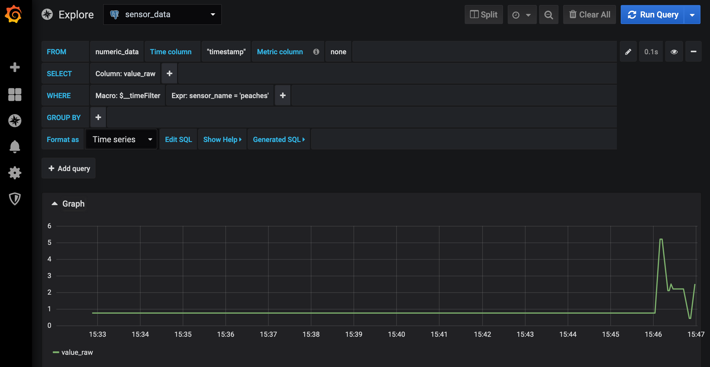Once connected, you can select the “Explore” option from the left navigation bar to bring up an interactive page for looking at data contents. If you select the sensor_data data source from the drop-down menu at the top, grafana will help you build a SQL query. In the line marked WHERE select the + to add an expression, click and replace the left value with sensor_name (the name of one of the columns in our table) and the right value with 'peaches' to view the time series of our peaches data. The full configuration and rendering should look something like

Feel free to explore the grafana UI, you can change the time interval or make various other changes. If you set new values to peaches, you’ll see the values in the plot change. Grafana also supports saving what it calls dashboards, which render one or more query. These can be saved and even added to its provisioning system (where they can be loaded automatically and even version controlled). Those capabilities are documented by grafana and are outside the scope of this guide.